Why Sample-Size Calculation Isn't Optional
Your team launches an A/B test on a new checkout flow. Three days in, the conversion rate looks promising. Someone checks the p-value: 0.04, below the 0.05 threshold. You ship the winner.
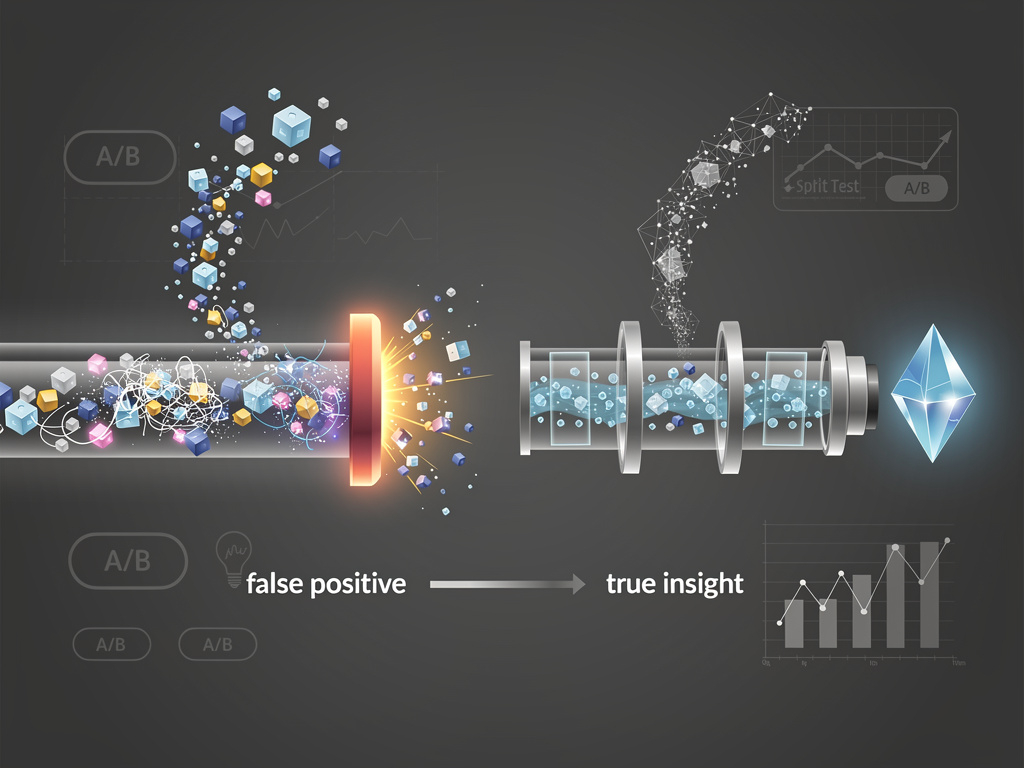
Two months later, revenue drops. The “winner” was a false positive. The real effect was negligible, but you caught a random fluctuation and acted on it.
This happens often in teams that treat sample-size calculation as optional paperwork. The consequences are measurable: false positives delay real insights and erode trust in data. Running tests longer than necessary wastes resources and slows down decisions that could have shipped weeks earlier. A survey by ABTestPro found that 60% of practitioners admit to peeking at results without applying statistical corrections, a habit that can inflate the false-positive rate from 5% to over 30%.
Frequentist and Bayesian frameworks both offer principled approaches to sample-size determination, but they answer different questions. Frequentist methods ask: “How surprising is this data if there is no effect?” Bayesian methods ask: “What is the probability of uplift given what we already know?” Neither question is wrong; they are simply not the same question.
If you've been treating sample-size calculation as a box to check, it's time to see how that approach wastes resources. Every valid experiment starts with three numbers that define the sample-size triangle. These parameters underpin both frameworks, but they lead to different interpretations of the results.
| Parameter | What it means | Typical target |
|---|---|---|
| Minimum Detectable Effect (MDE) | Smallest uplift worth acting on | 1-5% absolute lift for conversion |
| α (type I error rate) | Tolerated chance of a false positive | 0.05 (5%) |
| Power = 1 - β | Probability of catching a true effect of size MDE | 0.80 (80%) |
Changing any side forces an adjustment elsewhere: halve the MDE and you will need roughly four times the traffic because required sample size scales with 1/Δ².
The same three numbers create a divide in interpretation. A Frequentist p-value of 0.03 answers: If the true effect were zero, the chance of seeing data this extreme is 3%. A Bayesian posterior probability of 0.95 answers: Given the data and my prior beliefs, there is a 95% chance that Variant B is better.
Stakeholders often understand “95% chance of uplift” better than “p = 0.03,” but the two aren't interchangeable. Confusing them—treating a p-value as a posterior probability—causes many misinformed decisions. Keep the triangle clear and match your question to the framework that answers it. For Frequentists, these three numbers form a fixed contract before the first visitor arrives.
Frequentist Sample-Size Calculation: Power, MDE, and Fixed Horizons
Frequentist sample size derives from power analysis. The core question is: If a true effect of a specific size exists, how many observations do we need to detect it with 80% probability, while keeping our false positive rate at 5%? The resulting formula follows this structure:
n = ((Z₁₋α/₂ + Z₁₋β)² × [p₁(1−p₁) + p₂(1−p₂)]) / Δ²
Where Δ represents your MDE, p₁ and p₂ are baseline and treatment proportions, and the Z-values correspond to your chosen α and power thresholds. The math isn't optional; it shows how sample size scales with your choices, revealing the cost of demanding more certainty or smaller effects.
Consider the Minimum Detectable Effect. This is the smallest effect size worth detecting, the threshold below which you consider the business impact too small to matter. Here's the arithmetic: halving your MDE roughly quadruples your required sample size. The inverse square relationship means small effect sizes demand enormous traffic. If you are trying to detect a 1% lift on a 10% baseline conversion rate, you need roughly four times the traffic required for a 2% lift. This shapes business strategy; chasing tiny improvements in high-variance metrics can lead to month-long runtimes.
Traffic splits make this worse. A 90/10 split instead of 50/50 cuts your effective sample size for detecting differences. The variant with less traffic becomes the bottleneck, and the math penalizes this imbalance. Teams running uneven splits often don't realize they're wasting experiment traffic for operational convenience.
This creates rigidity by design. You must commit to sample size upfront, based on estimated traffic and effect size, before collecting data. Valid Frequentist inference requires a pre-registered, fixed sample size. Peeking without correction inflates false positives from 5% to 30% or higher.
Sequential fixes exist. Alpha-spending functions like O'Brien-Fleming and Pocock allow safe monitoring by adjusting significance thresholds across interim analyses. These preserve nominal error rates when followed rigorously, but they require pre-specification and discipline. Using them as post-hoc justification doesn't work; you can't decide to stop early after seeing the data.
The Frequentist framework demands upfront commitment. That rigidity isn't a bug; it's the mechanism that controls error rates. If your team struggles with pre-registration, the solution isn't to abandon the framework but to build processes that support it. But what if your team can't wait for that fixed horizon, or you have prior knowledge that should shape the experiment? This is where the Bayesian framework comes in, trading rigid pre-commitment for flexibility.
Instead of asking how surprising the data would be under a null hypothesis, Bayesian planning asks for the probability of uplift given what you already believe. It replaces power with assurance: the average probability of crossing a posterior-probability threshold (e.g., P(B > A) > 0.95) across the prior distribution of the effect. This shifts the focus from a fixed-n guarantee to a probabilistic guarantee that integrates prior belief.
Because assurance is evaluated over the prior, you can monitor continuously without inflating false positives, if you adhere to a decision-theoretic stopping rule such as expected loss or a highest-density-interval criterion. Naïve thresholds like “stop when P(B > A) > 0.95” can still bias error rates when the prior and the data conflict.
Prior choice directly shapes sample-size needs. Uninformative priors let the data dominate but often require larger samples, while informative priors can shrink needed n but demand rigorous justification. Computationally, <mark class=." data-type="AI Pattern">Computationally, modern libraries make MCMC or variational inference feasible for most A/B-test scales, though teams should benchmark latency against the speed gains of continuous monitoring. Yet this flexibility introduces a temptation that undermines both frameworks: the urge to peek at results and stop early when numbers look favorable, which creates a statistical trap.
The Peeking Problem: Error Control Under Continuous Monitoring
The peeking problem occurs when practitioners check results continuously without applying corrections. Naïve Frequentist monitoring inflates false positive rates because each peek is treated as an independent test when the sample size was calculated for a single analysis.
The numbers are stark. A test with a 5% false positive rate, checked daily for two weeks, can see that rate climb to 30% or higher. You are not accumulating evidence; you are accumulating opportunities for random fluctuation to trick you. ABTestPro's technical analysis shows how multiple looks compound this risk, turning a controlled experiment into a fishing expedition.
Frequentist solutions exist. Pre-specified interim analyses with alpha-spending functions preserve nominal α when followed rigorously. O'Brien-Fleming spending preserves most of your significance threshold for final analysis while allowing early stopping for overwhelming effects. Pocock spending uses more conservative thresholds throughout but permits more flexible monitoring. Both require pre-specification; deciding your analysis schedule before seeing any data.
Bayesian solutions also exist. Stopping rules based on posterior probability thresholds or expected-loss criteria maintain validity when declared before data collection. The key phrase is “when declared before looking at data.” Bayesian flexibility does not mean you can check whenever you want and stop whenever results look good; that is still p-hacking with posterior probabilities.
Hybrid tactics address both error control and stakeholder communication. Many teams run Frequentist sequential tests as the primary analysis for rigorous error control while reporting Bayesian posteriors for business communication. You get the statistical discipline of fixed-horizon testing with the intuitive interpretability of “92% probability of uplift.” This is not cheating; it is matching the tool to the audience.
The peeking problem reveals something important: neither framework is a silver bullet. Both require discipline. The most common failure mode is not choosing the wrong framework but implementing either without honoring its assumptions. One of the most critical assumptions in the Bayesian framework is the prior; its specification directly impacts sample size requirements and demands expertise that Frequentist methods do not require at the same step. This prior specification acts as a hidden lever that can dramatically shrink your required sample size or silently bias your results, depending on how carefully you wield it.
Optimistic priors reduce required samples but introduce bias if they misrepresent reality. This trade-off is significant and frequently overlooked in practice.
Weakly informative priors represent practical defaults for product experimentation. Consider conversion rates expected in the 5-15% range: a Beta(2,20) prior encodes enough structure to prevent pathological estimates while allowing data to dominate. This is not a cop-out; it is a principled choice that balances stability with learning.
Sensitivity analysis should be routine. Vary your prior hyper-parameters and observe how conclusions change. If your results flip based on reasonable prior adjustments, that is a signal your data is not carrying enough weight to support confident claims. Sensitivity analysis is essential; it separates rigorous Bayesian analysis from mere assertion.
Informative priors carry real risks. They can dramatically reduce required sample sizes, which sounds attractive until you realize you are essentially borrowing information from previous experiments. That borrowing introduces confirmation bias if the prior misrepresents the true baseline. Documentation and justification become essential operational requirements, not optional best practices.
roughly 47% of practitioners have encountered prior misspecification errors. That is not a small risk. Organizations adopting Bayesian testing without investing in prior expertise are trading Frequentist rigidity for Bayesian bias, a swap that only pays off if the new risks are managed. The real question is which framework's complexity your decision context can handle.
Decision Framework and Hybrid Implementation
Matching your statistical approach to your risk profile requires moving from philosophical debate to operational reality. The question is not “Which framework is correct?” but “Which framework serves this decision?”
High-stakes, irreversible decisions warrant Frequentist methods with sequential testing corrections. Pricing changes, regulatory compliance, and situations requiring strict error control need the error-rate guarantees that Frequentist power analysis provides. When the cost of being wrong is high and you cannot easily reverse course, the rigidity of fixed horizons and alpha-spending functions becomes a feature, not a bug. Small MDEs in these contexts demand the mathematical rigor that only careful power analysis can provide.
Rapid-iteration, low-stakes scenarios fit Bayesian methods with weakly informative priors and pre-specified stopping rules. UI tweaks, low-traffic features, and experiments where velocity outweighs occasional false-positive costs benefit from Bayesian flexibility. Here, the cost of delayed learning exceeds the cost of occasional errors. Bayesian continuous monitoring pays dividends you cannot capture with Frequentist rigidity, provided you have the expertise to specify and defend your priors.
Map economic weight explicitly. Ask: “What is the expected uplift if the variant wins? What is the cost of shipping a false positive?” When the cost of delayed learning exceeds the cost of occasional errors, Bayesian continuous monitoring dominates. When decisions are irreversible and errors are expensive, Frequentist fixed-horizon provides necessary caution. This mapping is not philosophical preference; it is operational decision-making that puts numbers on the trade-offs.
Hybrid workflows combine strengths. Use Frequentist sequential tests as primary analysis for error control, then overlay Bayesian posteriors for stakeholder communication. Some teams go further: Bayesian priors stabilize early-stage estimates in low-traffic scenarios while Frequentist error budgets govern final decisions. The best methodology is the one your team can implement honestly with proper stopping rules and pre-registration.
Implementation discipline matters more than the philosophical label you attach to your approach. Pre-register your stopping boundaries. Document your priors. Run automated interim analyses. These practices serve both frameworks. A correctly implemented framework outperforms a theoretically superior one that is executed poorly. Ultimately, both frameworks can produce sound inferences, but only when their specific assumptions are respected through disciplined execution.
Implementation Discipline Beats Framework Preference
That discipline matters more than the label on your approach. Both Frequentist and Bayesian sample-size calculations produce sound inferences when their assumptions are respected. The choice should be driven by decision context, not by a desire to win the methodological debate.
Actionable checklist
- Document MDE, α/power targets or prior/assurance thresholds up front.
- Pre-register stopping boundaries (fixed horizon, alpha-spending function, or Bayesian decision rule).
- For Bayesian tests, conduct a prior-sensitivity analysis and record the justification.
- Verify that any sequential Frequentist test uses a correctly implemented alpha-spending function.
- Communicate results with the appropriate uncertainty measure (p-value and confidence interval or posterior probability and credible interval) so stakeholders receive a clear, honest picture.
Better business decisions come from rigorous execution, not from choosing the 'right' statistical framework. Let discipline guide your experiments, and the numbers will follow.